10 Digital Terrain Analysis
Explain what a DEM is and how it is used
Derive topographic properties
Perform basic hydrological analysis
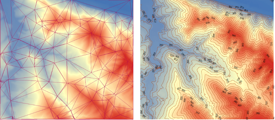
Digital terrain analysis (DTA) refers to spatial analysis methods and techniques applied to extract information about Earth’s surface from digital elevation data. By representing the landscape in a digital format Figure 10.1, GIS enables the quantitative analysis of topography, allowing researchers and practitioners to model surface processes and support decision-making. Typical applications of DTA span hydrological modeling, hazard (e.g., flood) assessment, ecological analysis, and urban planning. As such, terrain analysis forms a critical component of modern geospatial analysis and environmental science.
Digital Elevation Model (DEM): refers to digital cartographic representation of the elevation of the land at regularly spaced intervals in x and y directions, using z-values referenced to a common vertical datum. DEM usually refers to the bare-earth z-values.
Digital Surface Model (DSM): similar to DEM, depicts the elevations of the top surfaces of buildings, trees, towers, and other features elevated above the bare-earth.
Digital Terrain Model (DTM): in some countries, DTMs are synonymous with DEMs, representing the bare-earth terrain with uniformly spaced z-values, as in a raster.
As used in the U.S., a DTM is a vector dataset composed of 3D breaklines and irregularly spaced 3D mass points, typically created through stereo photogrammetry, that characterize the shape of the bare earth terrain. Breaklines more precisely delineate linear features whose shape and location would otherwise be lost.
In this case, a DTM is not a surface model and its component elements are discrete and not continuous; a TIN or DEM surface must be derived from the DTM.
10.1 Attributes derived from DEM
DTA is implemented on DEM in order to derive various terrain attributes include:
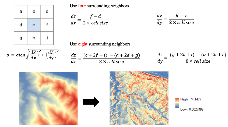
Slope – describes the maximum rate of change in value from each pixel to its neighbors, measuring the steepest direction of elevation change. In this case, the maximum change in elevation over the distance between the center cell and its eight neighbors identifies the steepest downhill descent from the cell Figure 10.2. The lower the slope value, the flatter the terrain; the higher the slope value, the steeper the terrain. Note that slope often does NOT fall parallel to the rater rows or columns.
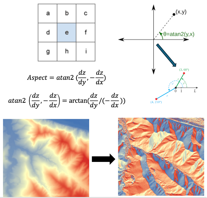
Aspect – calculates downslope direction of the maximum rate of change in value from each cell to its neighbors. It describes the direction of the slope, which is the direction that the slope ‘faces.’ In ArcGIS, Aspect is measured clockwise in degrees from 0 (due north) to 360 (again due north) in full circle Figure 10.3. Flat areas having no downslope direction are given a value of -1.
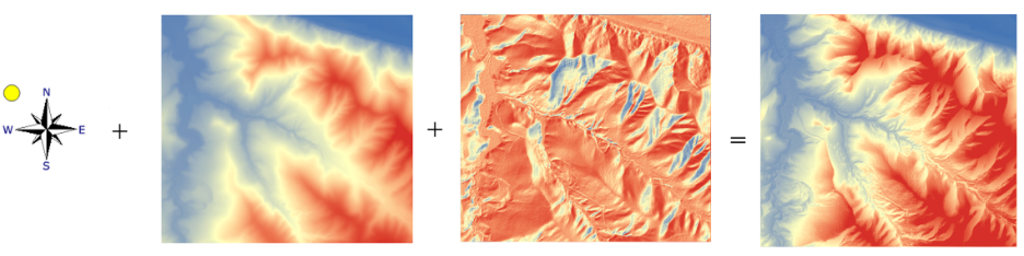
Hillshade – is a visualization technique that simulates the illumination of a surface by calculating light intensity values for each cell in a raster dataset. The resulting image represents variations in light and shadow as shades of gray, typically ranging from 0 (dark) to 255 (bright). This method enhances the three-dimensional appearance of terrain, making surface features easier to interpret Figure 10.4. Hillshade is particularly useful for analysis and cartographic display, especially when combined with transparency to overlay other spatial data.
Viewshed – determines which locations on a surface (raster layer) are visible from a set of observer points (additional layer). Using elevation data, the analysis evaluates line-of-sight between each observer and surrounding cells to identify visible areas. The output is a raster in which each cell is assigned a value indicating the number of observer locations from which that cell can be seen Figure 14.1. This allows users to assess visibility patterns across the landscape, which is useful in applications such as site planning, telecommunications, and landscape assessment.
Area solar radiation – calculates incoming solar radiation from a raster surface Figure 10.6. The method considers factors such as slope, aspect, surface orientation, and the position of the sun to estimate spatial variations in insolation. Because the calculation accounts for changes in solar angle over time and the effects of terrain shading, it can be computationally intensive, especially for large datasets or fine-resolution surfaces (can take hours to days!). This type of analysis is commonly used in studies of energy balance, vegetation patterns, and solar energy potential.
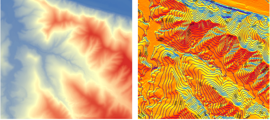
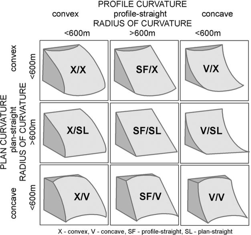
Curvature – describes the shape of the land surface and characterizes whether a slope is concave or convex Figure 10.7. Mathematically, curvature is derived by calculating the second derivative of the surface, often described as the “slope of the slope.” In hydrological analysis focusing on surface water, curvature determines acceleration/deceleration and convergence/divergence of flow across a surface. This measure helps identify areas where the terrain is bending upward (convex) or downward (concave), offering additional insight beyond slope and aspect in terrain analysis.
10.2 Hydrological analysis – surface water
Hydrological analysis in GIS can be divided into two broad categories, including surface water and ground water processes. While surface water analysis focuses on modeling the amount of water that travels downstream, ground water analysis deals with subsurface processes such as infiltration, drainage and recharge. Surface flow is directly affected by landscape topography, When gravity was the only force that drives flow of surface water. In this section, we will focus on surface water processes, whereas ground water dynamics require different data and modeling approaches.
Hydrological analysis focusing on surface flow aims to model the flow of water across a surface to understand where the (surface) water comes from and where it is flowing to. The primary objective is to extract hydrologic information and drainage system characteristics from a DEM.
Drainage system: is the area upon which water falls and the network through which it travels to ana outlet.
Watershed: aka drainage basin or catchment, is an area that drains water and other substances to a common outlet. Size of a watershed can vary across several geographical scales (e.g., a modest inland lake vs. Mississippi river watershed that spans 1.15 million square miles).
Pour point: is the point at which water flows out of an area. This is usually the lowest point along the boundary of the watershed.
Drainage network: is the network through which water travels to the outlet.
Ridge line: also known as a watershed divide, represents a boundary that separates adjacent drainage basins. Surface water does not flow across this boundary; instead, it is directed away from the ridge in opposite directions. As a result, flow is divergent at watershed divides.
Valley line: or drainage line, represents the lowest part of the terrain where water accumulates and flows downstream. Water from surrounding areas moves toward and along the valley line, often forming stream channels. At these locations, flow is convergent, as surface water concentrates into a defined pathway.
A typical hydrological analysis focusing on surface flow include condition DEM, flow direction, flow accumulation, stream threshold, place outlets, watershed.
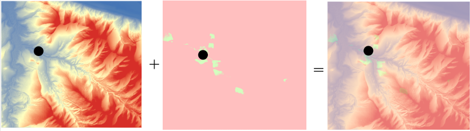
Condition DEM – the first step in applying hydrological analysis using DEM data is condition DEM or pit filling. This process is used to remove anomalies and erroneous values within a DEM to fill up water over depressions to force flow, because a derived drainage network may be discontinuous if sinks are not filled Figure 10.8. However, once applied, data and drainage are being altered. However, since pit filling changes the landscape artificially, special attention needs to be paid toward the characteristics of the terrain Figure 10.8.
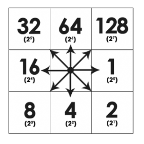
Flow direction – determines the direction of flow from every cell in the DEM. An eight-direction (D8) flow model (Jenson and Domingue 1988) is often used Figure 10.9. Again, we only model surface flow here, and the ground flow is different from the surface flow. Flow directions are hard to specify on flat land surface. To solve this, you need to either manually specify a flow direction applied to flat area, or use a larger cell size or neighborhood to calculate the flow.
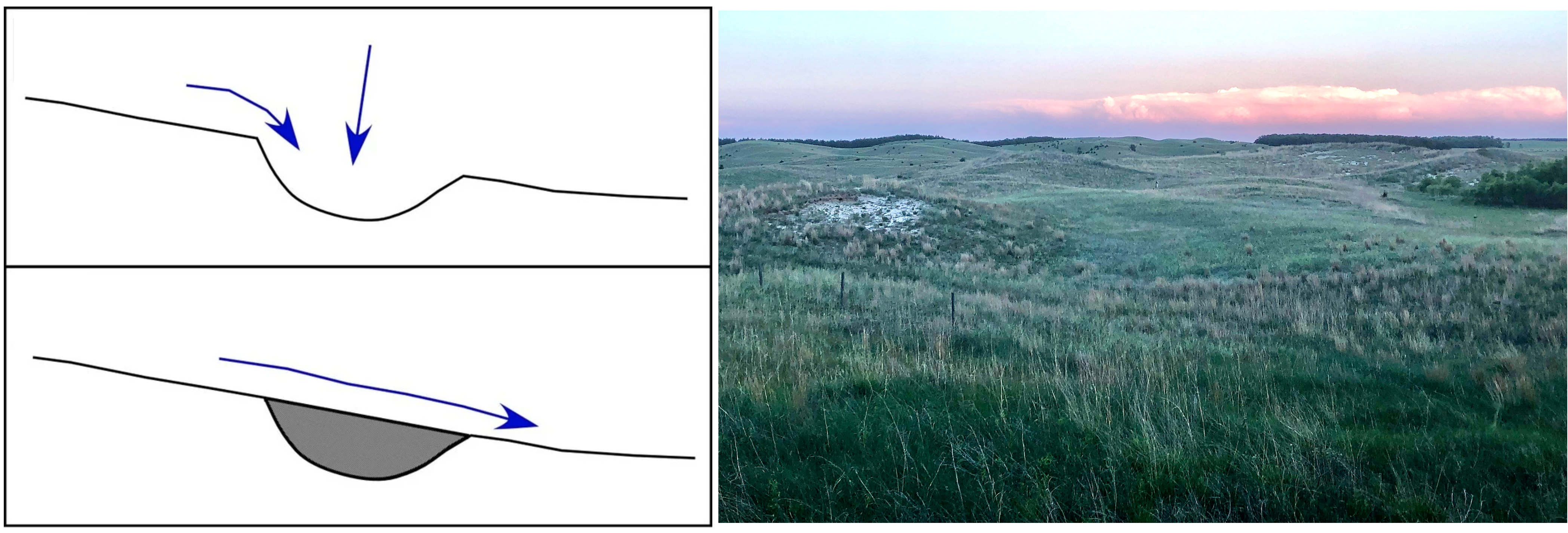
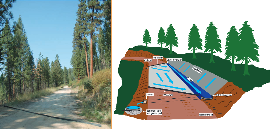
Note that built features (e.g., ditches, culverts) may alter flow directions that are not represented by terrain Figure 10.10.
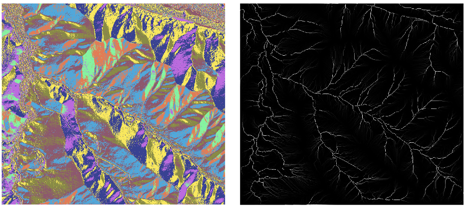
Flow accumulation – generates a raster of accumulated flow by counting accumulated weight of all cells flowing into each downslope cell Figure 10.11. Once the flow accumulation is calculated, a threshold can be applied to the flow accumulation result to identify stream networks. Note that the threshold is an arbitrary value that needs to be evaluated case-by-case.
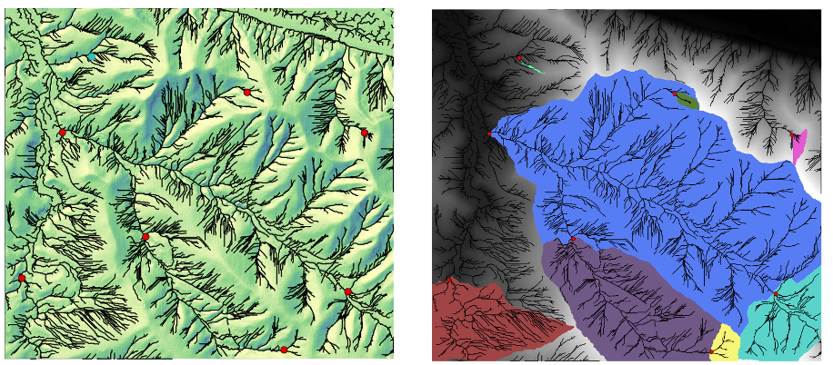
Pour point and watershed – A watershed is the upslope area that contributes flow to a common outlet as concentrated drainage. You need to specify pour point locations (outlets on streams) for which watersheds will be delineated Figure 10.12.
10.3 References
Black, Thomas A. and Luce, Charles H. 2013. Measuring water and sediment discharge from a road plot with a settling basin and tipping bucket. Gen. Tech. Rep. RMRS-GTR-287. Fort Collins, CO: U.S. Department of Agriculture, Forest Service, Rocky Mountain Research Station. 38 p.
Heidemann, Hans Karl, 2018, Lidar base specification (ver. 1.3, February 2018): U.S. Geological Survey Techniques and Methods, book 11, chap. B4, 101 p., https://doi.org/10.3133/tm11b4.
Jacoby, B., Peterson, E. and Dogwiler, T. (2011) Identifying the Stream Erosion Potential of Cave Levels in Carter Cave State Resort Park, Kentucky, USA. Journal of Geographic Information System, 3, 323-333. doi: 10.4236/jgis.2011.34030.
Szypuła, B. (2017). Digital Elevation Models in Geomorphology. In Hydro-Geomorphology - Models and Trends. InTech. https://doi.org/10.5772/intechopen.68447