5 Map Projection
Define map projection
Identify different types of map projections
Describe common distortions in map projections
Select appropriate map projections for given tasks or applications
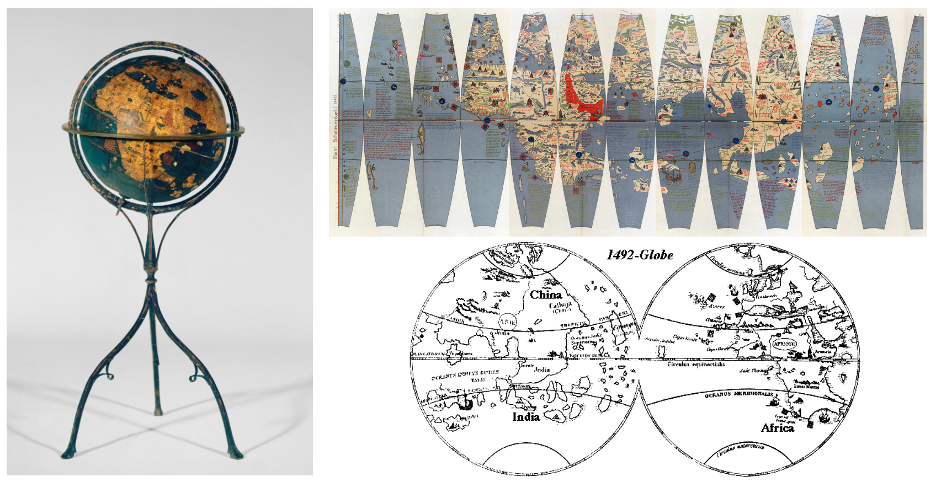
While a geographical coordinate system (GCS) provides an accurate way to locate any point on the globe, it’s not practical for many tasks. For example, it is impossible to accurately measure distances and areas directly from a sphere or ellipsoid. To perform tasks like land surveying, field work, navigation, and urban planning, we need a flat, two-dimensional map with linear units of measure (e.g., meters or feet). This is where map projections come in. A map projection is a mathematical transformation used to convert the three-dimensional, curved surface of a GCS into a two-dimensional, flat plane Figure 5.1. This process is necessary to create a usable map, but it’s also the source of all map distortion, because it is impossible to flatten a sphere without stretching or compressing some of its features. Every map projection introduces some type of distortion—whether in shape, area, distance, or direction. Different projections are designed to preserve one or more of these properties at the expense of others, which is why cartographers choose a specific projection based on the purpose of the map.
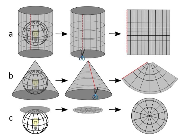
To make a map projection, cartographers need three foundational components: a developable surface, the aspect and points of tangency or secancy. These components define the geometric structure of the map projection. The developable surface is a geometric shape that can be flattened into a two-dimensional plane without any stretching or tearing. The most commonly used developable surfaces are the cylinder, plane (aka an azimuthal surface), and cone Figure 5.2. Each of these interacts with the globe in a unique way and is better suited to particular regions or mapping purposes. This initial step is what allows a curved surface to be represented on a flat map.
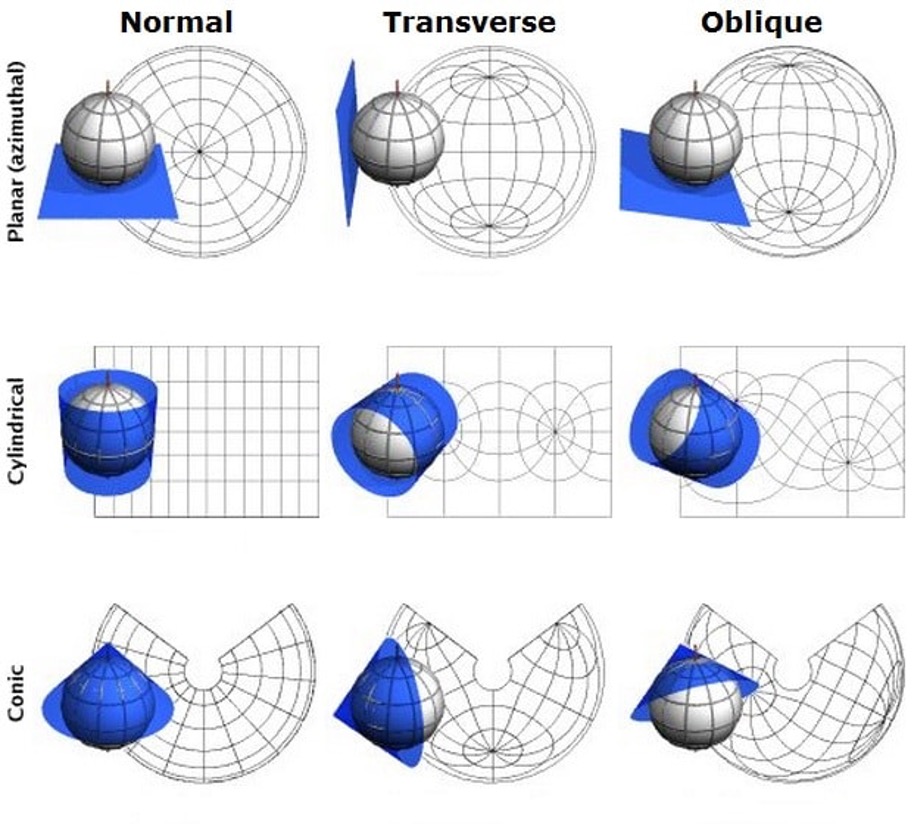
The aspect refers to the orientation of this developable surface in relation to the Earth’s axis of rotation. It determines how the surface is positioned Figure 5.3. The three main aspects are normal (aligned with the axis, such as a cylinder wrapped around the equator), transverse (perpendicular to the axis), and oblique (at an angle). The choice of aspect greatly influences the pattern of distortion and determines where the areas of least distortion will be on the final map. For instance, a normal cylindrical projection is most accurate near the equator, while a transverse one is better for a north-south region.
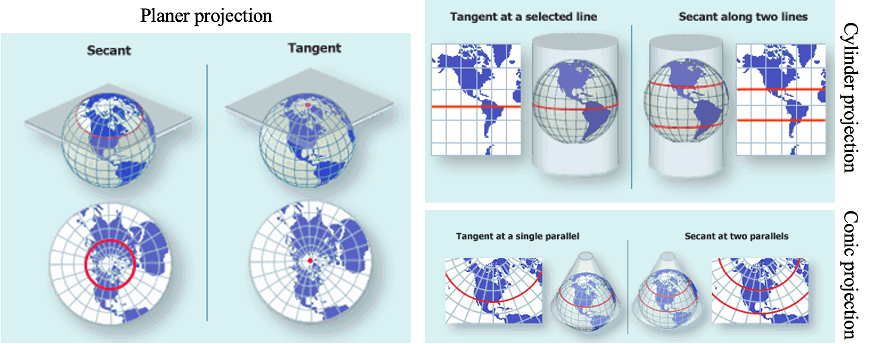
Finally, the points of tangency or secancy describe how the developable surface is positioned in relation to the globe Figure 5.4. A tangent projection touches the globe at a single point (for a plane) or a single line (for a cylinder or cone). A secant projection intersects the globe at two lines or circles. At these specific points or lines, the map scale is true, and there is no distortion, while distortion increases as one moves away from them. Secant projections tend to distribute distortion more evenly than tangent ones by spreading out the distortion across a larger area, as the scale is true at two separate lines. This makes them useful for regional maps where balance is important.
Together, these three components—developable surface, aspect, and contact points—define the structure of a projection and determine how faithfully the map represents the curved surface of the Earth. Understanding how they interact allows cartographers to choose the projection that best suits the purpose and geographic focus of the map.
5.1 Map projection types based on distortion
Map projections can be categorized based on the type of distortion they minimize or preserve. Since it is impossible to represent the curved surface of the Earth on a flat map without some distortion, cartographers choose projections depending on which geographic property—area, shape, distance, or direction—is most important to preserve for the map’s purpose. Based on the type of distortion they minimize, map projections are categorized into four main types: conformal, equal-area, equidistant, and azimuthal (aka true direction) projections Figure 5.5.
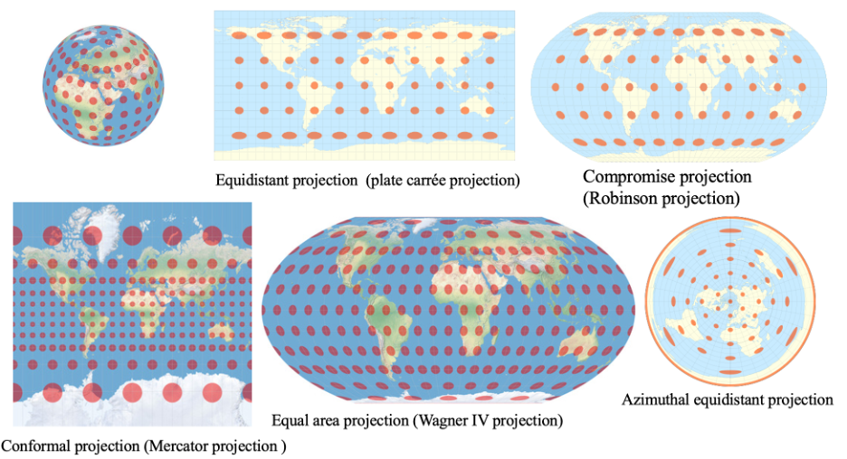
Conformal projection preserves angles and shapes locally. In these projections, the shape of small areas is maintained, but area and distance may be distorted. This means that at any point on the map, the angles are true, and the shapes of small features like coastlines and rivers are accurately represented. Thus, conformal projections are commonly used for navigational purposes because they represent compass directions accurately. However, this preservation of shape comes at the expense of area; landmasses may appear larger or smaller than they really are. The Mercator projection is the most famous conformal projection, widely used for marine navigation because it preserves compass directions. However, it greatly exaggerates the size of areas near the poles—for example, Greenland appears almost the same size as Africa, though it is much smaller in reality.
Equal-area projection preserves the relative sizes of landmasses and other features. These projections ensure that areas are represented in correct proportion, meaning that the proportions between countries, continents, or other regions are accurate in terms of area. This makes them useful for thematic or statistical maps where comparing sizes is important (e.g., population density or forest cover). To achieve this (preserve area), these projections must distort shapes, angles, and scale and the distortion of shape is generally more pronounced the farther a location is from the center of the projection.
Equidistant projectionpreserves distances from one or more specified points to all other points on the map. While they cannot preserve distances across the entire map, they are valuable when the focus is on a central location and its relationship to other places. As a result, equidistant projections are useful for applications like radio and seismic mapping where accurate distances from a central location are critical.
Azimuthal or true-direction projections preserve accurate directions from a central point to all other locations on the map. These are often used for air route maps or polar charts, where direction from the center is more important than shape or area accuracy. A common example is the azimuthal equidistant projection centered on the North Pole Figure 5.6, which shows all meridians as straight lines radiating from the center, making it easier to plot great circle routes—shortest paths between two points on a sphere.

In addition to these projection categories, compromise projection aims to balance distortion rather than preserving any single properties (area, shape, distance or direction) perfectly. Instead, compromise projection attempts to minimize overall distortion in all properties to produce a map that is visually pleasing and balanced in accuracy across the map. These projections are especially useful when the goal is to create general reference maps, such as world maps used in textbooks, atlases, or classrooms. For example, the Robinson projection, developed by Arthur H. Robinson in 1963, is one of the most widely used compromise projections. It was specifically designed to create a visually balanced representation of the entire world. On the Robinson map, the shapes and sizes of continents are moderately distorted, but the distortion is distributed more evenly across the map than in more specialized projections like Mercator. It avoids the extreme stretching of landmasses near the poles that occurs in conformal projections, and it presents continents like Africa and South America in proportions that are closer to reality. While the Robinson projection doesn’t preserve true scale, shape, area, or direction, its smooth, oval appearance and balanced distortions make it highly effective for thematic and general-purpose maps where no single property needs to be perfectly accurate. In fact, it was used by the National Geographic Society for nearly three decades as their standard world map projection.
It is important to remember that projection always introduce distortion. Each type of projection serves a different purpose and involves trade-offs between the various geographic properties. Choosing the right one depends on which characteristics are most essential for the map’s intended use.
5.2 Projected / Planar Coordinate Systems
Based on specific geographic coordinate system and map projection, a projected or planar coordinate system identifies locations by (x, y) coordinates (often in meters or feet) on a grid with equally spaced horizontal and vertical lines (Cartesian coordinates). Because mathematical calculations relating latitude and longitude to positions of points on a given map can become quite complicated, rectangular grids have been developed for the use of surveyors. In this way, each point may be designated merely by its distance from two perpendicular axes on the flat map. The Y axis normally coincides with a chosen central meridian, with y increasing north. The X axis is perpendicular to the Y axis at a latitude of origin on the central meridian, with x increasing east. X and Y coordinates are called “eastings” and “northings,” respectively. To avoid negative coordinates, we may have “false eastings” and “false northings” by adding constant values to all X and Y coordinates.
5.2.1 Projected coordinate system example 1: Universal Transverse Mercator Projection (UTM)
The Universal Transverse Mercator (UTM) projection is a widely used map projection system that applies a specific version of the Transverse Mercator projection on a global scale Figure 5.7. It is designed to provide a consistent and accurate way of mapping locations anywhere on Earth by dividing the planet into a series of zones, each with its own projection. The UTM system divides the Earth between 84°N and 80°S latitude into 60 vertical zones, each 6 degrees of longitude wide.
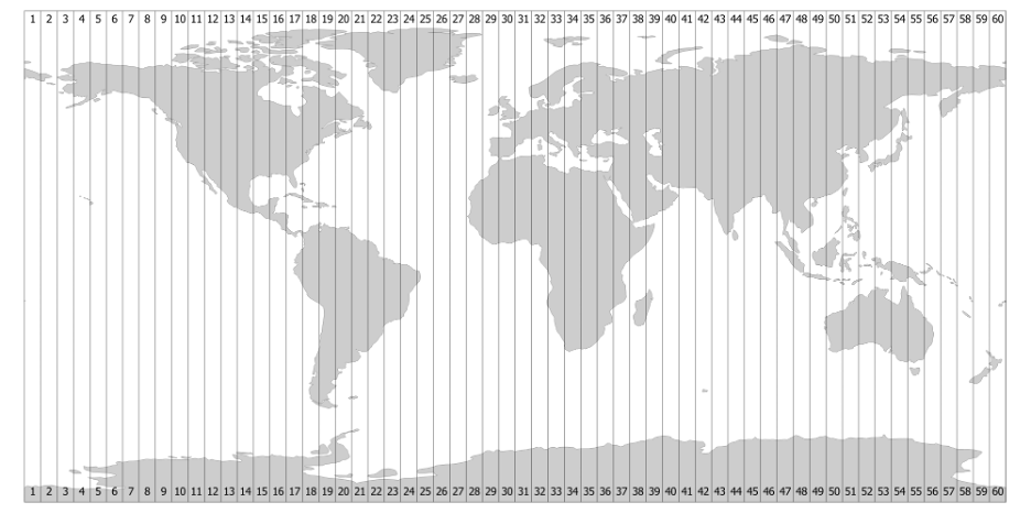
Each zone is projected individually using a Transverse Mercator projection, which means that the cylinder used for the projection is oriented longitudinally (north-south), rather than wrapping around the equator like in the regular Mercator projection. This “transverse” orientation minimizes distortion along a central meridian within each zone, making it suitable for mapping narrow north–south regions. To further reduce distortion, the UTM system uses a secant version of the Transverse Mercator projection, meaning the projection surface intersects the globe along two standard lines. This helps keep the scale distortion to a minimum within each zone—usually less than 1 part in 1,000. Each zone in the UTM system is assigned a unique number from 1 to 60, starting at 180° longitude and moving eastward. Additionally, the system uses Northing and Easting coordinates (measured in meters) rather than latitude and longitude. To avoid negative numbers, the equator is assigned a false northing of 10,000,000 meters in the southern hemisphere, and the central meridian in each zone is assigned a false easting of 500,000 meters. The UTM system is particularly useful for large-scale mapping because of its high positional accuracy over relatively small areas — typically within one UTM zone. However, because each zone is designed independently, maps that span multiple zones may require conversion or special handling to align correctly.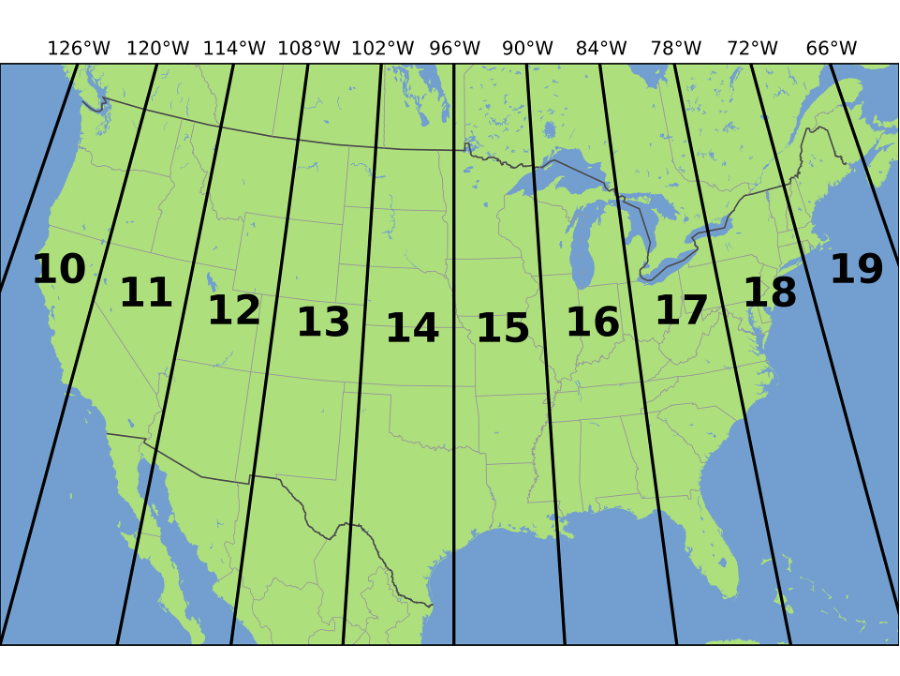
1)Determine the UTM zone
Zone = floor((Longitude + 180)/6) + 1
Central Median = Zone × 6 - 183;
2) Determine the (x, y) within the zone – Easting and Northing
Northing – number of meters north of Equator
Easting – number of meters east of central median of each zone
To avoid negative numbers:
False Easting: 500,000 m + Easting
False Northing (for southern hemisphere): 10,000,000 m + Northing
5.2.2 Projected coordinate system example 2: State Plane Coordinate System (SPCS)
State Plane Coordinate System (SPCS) is a grid-based system for determining coordinates of locations within the United States, designed in 1930s for large scale mapping of the US. It divides the US into over 120 zones, generally follow county boundaries, except in Alaska. Most states are divided into multiple zones—for example, Alaska has 10, Texas has 5, while Nebraska has only 1—to maintain high positional accuracy by limiting each zone’s geographic extent.
A baseline is set south of the zone and an origin meridian to the west of the zone and coordinates are eastings and northings in feet. Each zone has its own projection parameters, and the choice of projection depends on the general orientation of the zone. They can use different projections depending on the orientation of the state being projected and where it is located within the US. The Lambert Conformal Conic projection is usually used for east-west oriented zones (e.g., Tennessee) while Mercator projection is generally used for north-south oriented zones (e.g., Illinois). In some cases, the Oblique Mercator projection is used, particularly for certain zones in Alaska that do not align well with standard orientations.
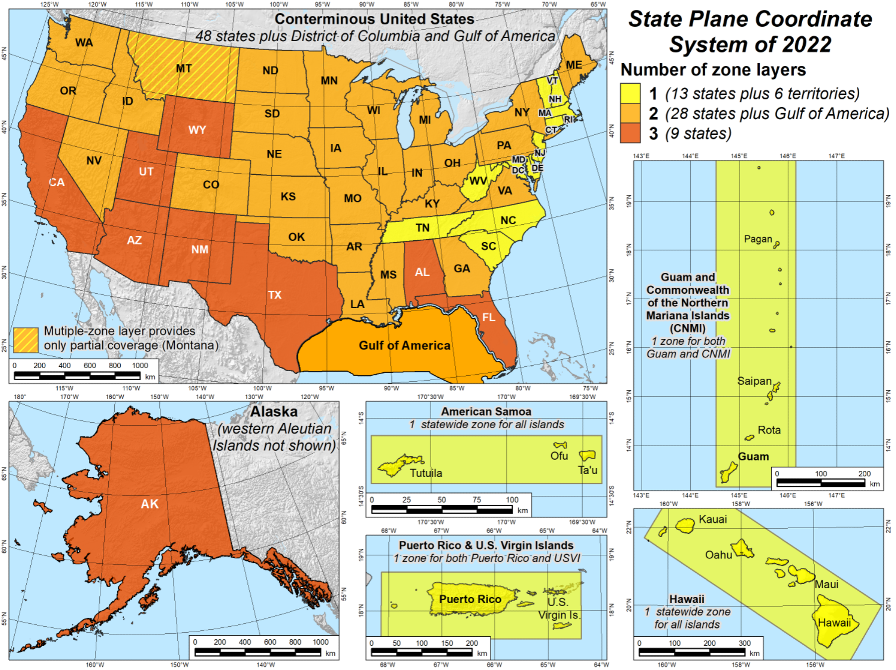
Note that a new generation of the SPCS (SPCS2022 Figure 5.8) will be released as part of Natioal Geodetic Survey (NGS) National Spatial Reference System (NSRS) Modernization. In SPCS2022, every U.S. state and territory will have a statewide zone. Most states include a statewide layer composed of multiple zones that collectively cover the entire state. In some cases, additional multi-zone layers are defined for only specific regions within a state. Beyond state-level zones, there are also “special use” zones that extend across the boundaries of multiple states. The variation in the number and configuration of zones reflects the active involvement of stakeholders during the SPCS2022 design process. Many states contributed input by submitting formal requests or proposals for zone definitions.
Maps are tools, and like any tool, the best one for the job depends on the task. This is NOT just a theoretical problem. Every map, from a web map to a printed atlas, is a conscious choice to use a particular projection to serve a specific purpose. For the scenarios below: which properties of a map projection would be most critical for you to preserve, and why?
Scenario 1 The Global Shipping Company. “You need to plan the most efficient routes for cargo ships traveling from Asia to the Americas.”
Scenario 2 The UN Climate Change Committee. “You are creating a map to show the global impact of rising sea levels.”
Scenario 3 The National Geographic Magazine Cartographers. “You are creating a detailed map of the continent of Africa for an educational atlas.”
5.3 References
Manson, S. M. (ed) (2025). Mapping, Society, and Technology. Second Edition. Minneapolis, Minnesota: University of Minnesota Libraries Publishing. URL: https://open.lib.umn.edu/mapping
PROJ contributors (2026). PROJ coordinate transformation software library. Open Source Geospatial Foundation. URL https://proj.org/. DOI: 10.5281/zenodo.5884394